Plotting multiple time series in a single plot

Recently a person posed a question on Stackoverflow about how to combine multiple time series into a single plot within the ggplot2 package. The question referenced another Stackoverflow answer for a similar type of question, but the person who posted the new question wasn’t able to apply the other answer in a way that produced the desired chart.

As specified in the question, data for various stock symbols is loaded into R via the quantmod::getSymbols() function, where the adjusted closing stock prices are extracted and saved to a vector.

library(quantmod)
library(TSclust)
library(ggplot2)
# download financial data

symbols = c('ASX', 'AZN', 'BP', 'AAPL')
start = as.Date("2014-01-01")
until = as.Date("2014-12-31")

stocks = lapply(symbols, function(symbol) {
    adjust = getSymbols(symbol,src='yahoo', from = start, to = until, auto.assign = FALSE)[, 6]
   names(adjust) = symbol
    adjust
  })

At this point the symbols object is a list that contains four xts (extensible time series) objects.

Code to produce a qplot() based on the Stackoverflow answer referenced in the question generated an error.

qplot(symbols, value, data = as.data.frame(stocks), geom = "line", group = variable) +
 facet_grid(variable ~ ., scale = "free_y")

> qplot(symbols, value, data = as.data.frame(stocks), geom = "line", group = variable) +
+   facet_grid(variable ~ ., scale = "free_y")
Error: At least one layer must contain all faceting variables: `variable`.
* Plot is missing `variable`
* Layer 1 is missing `variable`
Run `rlang::last_error()` to see where the error occurred.

The qplot() fails because there is no column called variable in the data that is passed to the plot function. Additionally, in order to produce the desired chart we need to extract the dates from the xts objects generated by quantmod::getSymbols() so we can use them as the x axis variable on the chart.

A solution with Base R

With a few adjustments, the code posted in the original question can be edited to produce the desired results.

Convert the xts objects to objects of type data.frame
Rename columns and save the stock ticker symbols as a distinct column, resulting in a wide format tidy data frame
Extract the rownames() that represent the time periods into another column

The revised code produces a list of data frames, one per stock ticker.

stocks = lapply(symbols, function(symbol) {
  aStock = as.data.frame(getSymbols(symbol,src='yahoo', from = start, to = until,
                                    auto.assign = FALSE))
  colnames(aStock) <- c("Open","High","Low","Close","Volume","Adjusted")
  aStock$Symbol <- symbol
  aStock$Date <- as.Date(rownames(aStock),"%Y-%m-%d")
  aStock
})

We use rbind() to consolidate the list into a single data frame.

  stocksDf <- do.call(rbind,stocks)

We use a combination of qplot() and helper functions from the ggeasy package to customize how the dates are rendered as x axis labels.

library(ggeasy)
qplot(Date, Adjusted, data = stocksDf, geom = "line", group = Symbol) +
     facet_grid(Symbol ~ ., scale = "free_y") +
     scale_x_date(date_breaks = "14 days") +
     easy_rotate_x_labels(angle = 45, side = "right")

Having corrected the errors in the original code, the qplot() produces the desired output.

An xts-friendly solution

One of the wonderful but sometimes frustrating aspects of R is that there is always more than one way to accomplish a given task, and plotting multiple time series on a single chart is no exception.

A day after I answered the question, Joshua Ulrich, one of the authors of the xts package, posted an answer that solves the problem in a manner that uses the xts objects in a manner more consistent with their original design.

Key differences in the two solutions include:

Load the stock ticker data into an environment, and then use merge() with lapply() to combine only the adjusted closing stock prices from all objects in the environment into one xts object
Remove .Adjusted from the column names via gsub()
Convert the xts object to a long form tidy data frame via ggplot2::fortify()

The fortify() function converts a model object to a data frame, and the melt = 'TRUE' argument converts the data from wide format to long format.

library(quantmod)
library(ggplot2)

symbols <- c("ASX", "AZN", "BP", "AAPL")
start <- as.Date("2014-01-01")
until <- as.Date("2014-12-31")

# import data into an environment
e <- new.env()
getSymbols(symbols, src = "yahoo", from = start, to = until, env = e)

# extract the adjusted close and merge into one xts object
stocks <- do.call(merge, lapply(e, Ad))

# Remove the ".Adjusted" suffix from each symbol column name
colnames(stocks) <- gsub(".Adjusted", "", colnames(stocks), fixed = TRUE)

# convert the xts object to a long data frame
stocks_df <- fortify(stocks, melt = TRUE)

The data frame generated by fortify() contains three columns, Index representing a date, Series representing the stock ticker, and Value, representing the Adjusted closing price on a given date.

> head(stocks_df)
       Index Series    Value
2014-01-02    AZN 19.53932
2014-01-03    AZN 19.63607
2014-01-06    AZN 19.64608
2014-01-07    AZN 19.51931
2014-01-08    AZN 19.52265
2014-01-09    AZN 19.80621

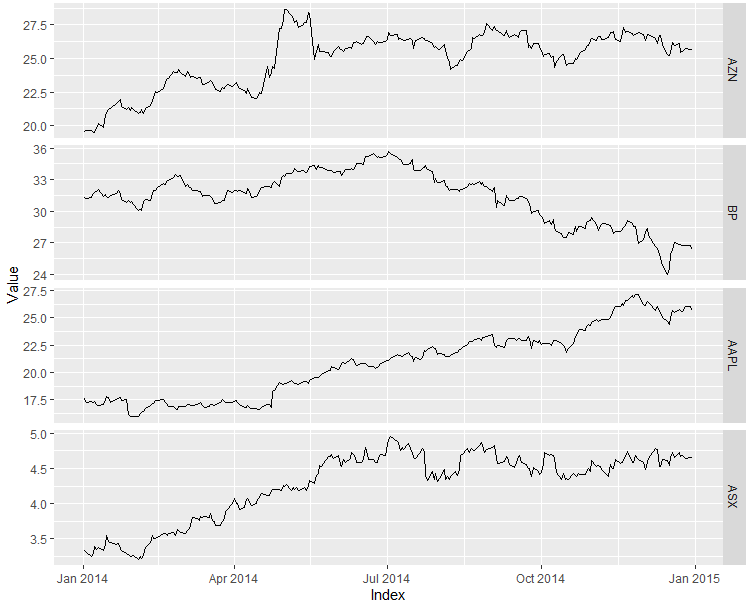
The last step in the process is to generate the facetted qplot().

# plot the data
qplot(Index, Value, data = stocks_df, geom = "line", group = Series) +
  facet_grid(Series ~ ., scale = "free_y")

Observations

I’m not a frequent user of quantmod. The fact that getSymbols() returns xts objects where the column dimension includes a ticker symbol along with the actual column name has led me to use lapply() to separate the ticker names from the columns and immediately convert the objects to data frames, an object type with which I am more familiar.

Joshua’s solution helped me realize that by retaining the xts object type and using merge(), I can avoid converting row names to a date column and defer separation of the stock ticker symbol from the column name.

Second, R is constantly changing. As I reviewed Joshua’s code, I discovered that ggplot2::fortify() is being deprecated. The current tidyverse function that replicates the behavior of fortify() is broom::tidy(), and it enables us to avoid the gsub() step because it automatically tidies the column names.

stocks <- do.call(merge, lapply(e, Ad))
head(stocks)

> head(stocks)
           AZN.Adjusted BP.Adjusted AAPL.Adjusted ASX.Adjusted
2014-01-02     19.53932    31.31375      17.65500     3.338105
2014-01-03     19.63607    31.24196      17.26720     3.302056
2014-01-06     19.64608    31.32681      17.36135     3.244379
2014-01-07     19.51931    31.68575      17.23719     3.287637
2014-01-08     19.52265    31.80323      17.34635     3.395782
2014-01-09     19.80621    31.88154      17.12484     3.352525

library(broom)
a_tibble <- tidy.zoo(stocks)
head(a_tibble)
> head(a_tibble)
# A tibble: 6 x 3
  index      series value
  <date>     <chr>  <dbl>
1 2014-01-02 AZN     19.5
2 2014-01-03 AZN     19.6
3 2014-01-06 AZN     19.6
4 2014-01-07 AZN     19.5
5 2014-01-08 AZN     19.5
6 2014-01-09 AZN     19.8

I’m grateful that Joshua took the time to post an answer to this question because I learned some things from him, and in the future I’ll be less likely to immediately convert xts objects to data frames when I work with time series.